- Add a sink destination by selecting the + sign in the lower right of the Select transformation ➢ select Sink from the pop‐out menu ➢ enter an output stream name (I used Brainwaves) ➢ create a new dataset for the deduplicated brain waves (for example, BrainwavesJson), as you did in step 3, but this time leave the File text box empty ➢ select the Data Preview tab ➢ and then click Refresh. Notice that the four duplicates are not part of the result, as shown in Figure 6.47.
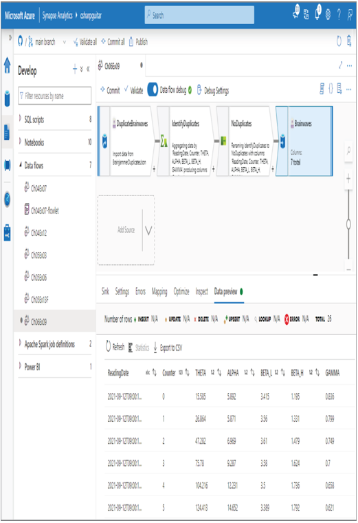
FIGURE 6.47 Handle duplicate data—data flow sink
- Click the Commit button, and then click the Publish button.
The first change you may have noticed in Exercise 6.9 versus some of the others has to do with the data. In order to get this ingestion to flow into the tool, the data needed to be in a different structure. For this example, the data was changed manually. In the real world you could have performed some data transformation to evolve from the JSON file format you have seen up to now to the one used in Exercise 6.9. Either way, the point is that you will likely receive data in many different formats, and you will likely need to format it into a structure that aligns with the requirements of the feature you want to use.
In Exercise 6.9 you used some transformations that have not yet been covered. You have already been exposed to Source and Sink, so there is no need to cover them in detail, other than reaffirming that the source is where the data is ingested from, and the sink is where you want to write the transformed data to. The Data Preview tab from the source, as shown in Figure 6.43, resembles the following:
Exercise 6.9 introduced a new transformation: an Aggregate transformation. The action you took in this transformation was to identify the columns that the data would be grouped by. Because the intent was to find duplicates of the entire reading, all the columns were included, as shown in Figure 6.44. Then you added a new column named Readings that counted the number of matching readings with the same ReadingDate, as shown in Figure 6.45.
This technique is an interesting approach to filter out duplicate data. It did not remove any data from the file; instead, it grouped together matching entries and added a column that contained the count of matching readings.
The Data Preview tab of the Aggregate transformation resembles the following. Notice that instead of having three rows for the reading with a counter of 5, there exists only a single row. Similar for readings with counter 11 and 21. Note that some of the data had to be modified to fit on the page, but you should get the point.
Then, in the next transformation, the Select transformation, you selected only those rows in the group by output, without the count that resulted in only 26 rows being selected from the 30. Recall that the output of the Aggregate transformation’s Data Preview tab had only 26 rows, with an extra column that contained the number of duplicates, but still only one row of that specific duplicated data. So, when the Select transformation was run, you received only those 26 deduplicated rows, as summerized here.
This is a very interesting technique and one that can be applied in other places in your data analytics processes.